MCom I Semester Managerial Economics Baumol & Marris Models Study Material Notes

MCom I Semester Managerial Economics Baumol & Marris Models Study Material Notes:  Baumol Sales or Revenue Maximisation Model Theory Baumol Static Model Explanation of the Model criticism or Limitation so the Model Assumptions of the Marris Model Explanation of the Model Criticisms of the Marris Model

CTET Paper Level 2 Questions Answer Language II English Model paper

BAUMOL AND MARRIS MODELS

The operations of modern firms are so complex that they can not think about profit maximisation only. Their main problems are related to control and management. Their management is carried-out not by entrepreneurs but by managers and share holders. Shinc ownership and control in modern firms is in the hands of different persons, it is unrealistic to accept that the sole objective of modern firms is profit maximisation. Therefore, economists have propounded a number of theories of the firm. These are based on different objectives and classified under three categories :

(i) Managerial, (ii) Behavioural, and (iii) Agency Theories.

Baumol’s sales or revenue maximisation Model is a well known managerial theory of the firm. This is discussed as under:

BAUMOL’S SALES OR REVENUE MAXIMISATION MODEL (THEORY)

W.J. Baumol suggested sales or revenue maximisation as an alternative objective to profit maximisation’. He presente two basic models : the

First is a single-period static model, and the second is a multi-period dynamic model of growth of sales revenue maximisation. Each model has two versions, one without and one with advertising activities.

Rationalisation of the Sales-Maximisation Hypothesis Baumol offers several justifications of sales maximisation as a goal of the firm. Some of these are:

1 Salaries and other slack earrags of top managers are correlated more closely with sales than with profits.

2. The banks and other finanicial institutions keep a close eye on the sales of the firms and are more willing to finance firms with large and gowing sales.

3. The employees at all levels can be given higher earnings and better terms of work in general.

4. Large sales, growing over time, give prestige to the managers, while large profits go into the pockets of shareholders or owners.

5. large, growing sales strengthen the power to adopt competitive tactics.

BAUMOL’S STATIC MODEL

Baumol Model is based on the following assumptions:

1 There is a single period time horizon of the firm.

1.WJ. Baumol: Business Behaviour, “‘Value and Growth”, Macmillan, New York, 1959. ms at maximising its total sales revenue in the long run the current

2. The firm aims at maximisin subject to a profit constraint.

3. The firm’s minimum p the current market value of tis shares.

4. The firm is oligopolist demand curve is downward sloping the conventional type. in s minimum profit constraint is set competitively in terms of firm is oligopolistic whose cost curves are U-shaped and the is downward sloping. It total cost and revenue curves are also of

EXPLANATION OF THE MODEL

Baumol’s findings of oligopoly firms in America reveal that they follow sales maximisation objectives. He cites evidence to suggest that short-run revenue maximisation may be consistent with long-run profit maximisation. But saics maximisation is regarded as the short-run and long-run objective of the management. Let us take a model without advertising first :

Baumol’s model of sales maximisation with out advertising points out that the profit maximisation output 0Q will be smaller than the sales-maximisation output OD, and price higher than under sales maximisation. The reason for a lower price under sales maximisation is that both total revenue and total output are equally higher while under profit maximisation, total ouput is much less as compared to toal revenue.

Baumol & Marris Models

(b) Model with Advertising

Raumol’s model with advertising is illustrated in figure 2, where expenditure on advertising is taken on the horizontal axis and total revenue the vertical axis. TR is the total revenue curve. The 45° line AdC is the Advertisement cost curve. By adding a fixed amount of other costs equal to OC to the AdC curve, we get the total cost curve TC. Here production costs OC are assumed independent of advertising costs. TP is the total profit curve which is the difference between the TR curve and the TC curve. MP is the minimum profit constraint line. The profit maximisation firm will spend OQ on advertising and its total revenue will be OS (QA). On the other hand, given the profit constraint MP, the sales maximisation firm will spend OD on advertising and earn OT EDE) as the total revenue. Thus the sales-maximisation firm spends more on advertising (OD) than the TP and also earns higher revenue (DE) than the latter (QA), DE>QA, at the profit constraint MP. Thus it will always pay the sales maximiser to increase his advertising outlay until he is stopped by the profit constraint.

(c) Baumol’s Dynamic Model

In the Baumol’s dynamic model the time (-) horizon is extended and the profit constraint is endogenously determined. This is called as “multiperiod model”. The predictions of the multi-period model, according to Baumol are the same as those of the static period model.

Conclusion of the Model This model leads to the conclusion that a sales-revenue maximisation firm (i)will keep low prices, (ii) will produce at a higher level and (iii) will invest in such a manner, as on advertisement, that the demand for its product will increase.

Baumol & Marris Models

CRITICISMS OR LIMITATIONS OF THE MODEL

Bumol’s sales-revenue maximisation model is not free from certain weaknesses:

(1) Rosen berg has criticised that it is difficult to specify exactly the relevant profit constraint for a firm. He suggests so long as profits exceed the constraint, they will always be converted into advertising to increase sales.

(2) According to Shepherd, under oligopoly a firm faces a kinked demand curve and if the kink is large enough, total revenue and profits would be the maximum at the same level of output. So both the sales maximiser and the profit maximiser would not be producing different levels of output.

(3) Hawkins has shown that Baumol’s conclusion that a sales-maximiser will in general produce and advertise more than a profit-maximiser is invalid.

(4) Williamson has shown that sales maximation yields different results from profit maximisation, while in the case of multi-products, Baumol has argued that revenue and profit maximisation yield the same result.

(5) The model fails to explain not only actual competition but also the threat of potential competition from rival oligopolistic firms.

Despite the above-said limitations, there is no denying the fact that sales maximistion forms an important objective of modern firms in the present day business world.

Robin Marris in his book The Economic Theory of Managerial capitalism (1964) has developed a dynamic balanced growth maximising model of a firm. He cites the proposition that modern big firms are managed by managers and the shareholders are the owners who decide about the management of the firms. The Managers aim at the maximisation of the growth rate of the firm and the share holder (owners) aim at the maximisation of their dividends and share prices. To extablish a link between such a growth rate and the share prices of the firm, Marris develops a balanced growth model in which the manager chooses a constant growth rate at which the firm’s sales, profits, assets, etc. grow. If he chooses a higher growth rate, he will have to spend more on the advertisement and on Research and Development (R&D) in order to create more demand and new products. He will therefore retain a higher proportion of total profits for the expansion of the firm. As the managers are concerned more about their job security and growth (expansion of the firm, they will choose that growth rate which maximises the market value of shares, gives satisfactory dividends to share holders. On the other hand, the shareholders also want balanced growth of the firm because it ensures fair return on their capital. Thus the objectives of the managers may coincide with that of share holders (owners) of the firm and both try to achieve balanced growth of the firm.

ASSUMPTIONS OF THE MARRIS MODEL

The Marris model is based on the following assumptions:

1 It assumes a given price structure.

2. Production costs are given.

3. There is no oligopolistic interdependence.

4. There is no oligopolistic interdependence.

5. Factor prices are constant.

6. Firms are assumed to grow through diversification.

7. All major variables such as profits, sales and costs are assumed to increase at the same rate

Baumol & Marris Models

EXPLANATION OF THE MODEL

Given these assumptions, the objective of the firm is to maximise its balanced growth rate, G. The Gitself depends on two factors: first, the rate of growth of demand for the firm’s product, GD; and second, the rate of growth of capital supply, GS. Thus G = GD = GS.

Despite the fact that in modern big firms ownership is divorced from management, owners and managers have a common goal of balanced growth of the firm. According to Marris, there are two different utility functions for the manager and the owner of the firm. The utility function of the manager consists of his emoluments, status, power, job security, etc. On the other hand, the utility function of the owner ineludes profits, capital, output, market share, etc.

Thus, the manager of a firm aims a maximising his utility, and his utility depends upon the rate of growth of the firm. Though promoting the growth of the firm is the main objective of the manager, yet he is also motivated by his job security. The manager’s job security depends upon the satisfaction of shareholders who are concerned to keep the firm’s share prices and dividends as high as possible. Thus the manager aims at maximising the rate of growth of the firm and the shareholders (owners) aim at maximising their profits in the form of dividends and share prices. Marris analyses the means by which the firm tries to achieve its growth-maximisation goal. The firm may grow in size through the creation of new products which create new demands. Marris calls it differentiated diversification. The introduction of new products depends upon the rate of diversification, advertising expenses, R & D expenditures, etc.

Marries establishes the relationship between growth and profits on the demand side through diversification into new procducts. The links between growth and profits are different at different levels of growth. In this gorwth-profits relationship, growth determines profits.

Thus the firm expands (grows) and profits increase. With the further increase in the growth rate dut to grater diversification into new products, the growth-profitsrelationship becomes negative. This becuase there is the managerical constraint which sets a limit on the rate of managerial growth that restricts the growth of the firm. The firm’s managerial ability to cope with a great number of changes at once is limited. It is not possible to develop a larger management team for the development and marketing of new products. The higher rate of diversification requires higher expenditures on advertising and R & D, as a result, beyond a certain growth rate, the higher growth rate leads to a lower rate of profit. This illustrated in Figure 2 where the GD curve first rises, reaches the highest point M and then starts falling.

The other aspect of the growth-profits relationship is the rate of growth of capital supply. The aim of the shareholders is to maximise the growth rate of capital stock. The main source of finance for its growth is profits. Thus profits determine growth on the supply side. A higher level of profits provides more funds directly for reinvestment.

This gives a direct and positive relationship between profits and growth. this is shown in Fgiure 2 as a straight line GS from the origin.

For the equilibrium of the firm, the growth-demand and growth supply relationship must be satisfied.

GD This is achieved when the two curves GD and GS intersect at a point where the growth-profits combination gives the optimum solution. Suppose in the GD curve at point M where profits are maximised. This point does not provide an optimum solution because the managers desire more growth than is consistent with long-run profit maximisation. The extent to which they can increase the growth rate beyond point M depends upon their desire for job security. Their job security is threatened if the shareholders feel that the share! prices and dividends are falling and there is the threat of takeovers by other firms. This will affect the growth rate of capital supply (GS). thus it is the financial constraint which sets a limit to the growth of the firm on the.

Following Marris, it is the retention ratio which determines the growth rate of capital supply. The retention ratio is the ratio of retained profits to total profits. If this ratio is very low, it means that almost all profits have been distributed to the share holders. As a result, these are limited funds available with the managers for the growth of the firm and the growth rate will be very low. The gorwth-supply curve will be GS, as in fig. 2. By this curve firm’s equilibrium will be at point L. But this is again not the optimal equilibrium point of the firm because at L, the growth rate is low and profits are below the maximum level.

According to Marris, point E is the optimal equilibrium point of the firm. If the managers adopt a higher retention ratio than this point, the distributed profits will fall further and the share holder (owners) will not satisfied. The existing shareholders may decide to replace the managers.

Baumol & Marris Models

CRITISIMS OF THE MARRIS-MODEL

1 Marris assumes a given price structure for the firms. He does not explain how the prices of products are determined in the market.

2. Marris model ignores the problem of Oligopolistic interdependence of firms in a non-collusive market’.

3. According to Koutsoyiannis, Marris’s model is applicable basically to those firms which produce consumer goods. The model is not appropriate for analysing the behaviour of manufacturing businesses or Traders.

4. The assumption that all major variables such as profits, sales and costs in the crease at the same rate is highly unrealistic.

5. This model also does not analyse interdependence created by non-price competition.

Comparison of Marris’s model with Baumol’s Sales Maximisation Model:

Both models belong to the “managerialist school” of thought. In both models, managers deviate from the objective of profit maximisation. Both models assume a given price structure.

But in Baumol’s model managers are interested only in their own utility and in Marris’s model under conditions of steady growth managers can attain contemporaneously the maximisation of their own utility and of the utility of owners or shareholders.

Baumol & Marris Models

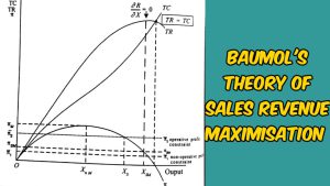
(a) Model without Advertising :

Baumol’s model without advertising is illustrated in Figure 1 where TC is the total cost curve, TR the total revenue curve, TP the total profit curve and MP the minimum profit or profit constraint line. The firm maximises its profits at 0Q level of output corresponding to the highest point B on the TP curve. But the aim of the e firm is to maximise its sales rather than profits. Its sales maximisation output is OK where the total revenue 5 KL is the maximum at the highest FM point of TR. This sales maximisation output OK is higher than the profit maximisation output 0QBut sales maximisation is subject to minimum Suppose the minimum profit level of the firm is represented by the line MP. the output OK will not maximise sales as the minimum profits OM are not being covered by total profits KS. For sales maximisation, the firm should produce that level of output which not only covers the minimum profits but also give the highest total ravenue consistent with it. This level is represented by OD level of output where the minimum profits DC (=OM) are consistent with DE amount of total revenue at the price DE/OD. (i.e., total revenue total output)